It is a “Hello, World!” program in FEniCS that solves following boundary-value problem.
Reference
Mathematical problem formulation
\[- \nabla^2 u(\boldsymbol{x}) = f(\boldsymbol{x}), \boldsymbol{x} \text{ in } \Omega, \\ u(\boldsymbol{x}) = u_D(\boldsymbol{x}), \boldsymbol{x} \text{ on } \partial\Omega.\]Where $u=u(\boldsymbol{x})$ is the unknown function, $f=f(\boldsymbol{x})$ is a prescribed function, in 2D with coordinates $x$ and $y$, the Poisson equation can be written as
\[-{\partial^2 u \over \partial x^2} - {\partial^2 u \over \partial y^2} = f(x,y).\]Steps in FEniCS
- Identify the compiutational domain $\Omega$, the PDE, its boundary conditions, and source term $f$.
- Reformulate the PDE as a finite element variational problem.
- Write a Python program which defines the computational domain, the variational problem, the boundary conditions, and source terms, using the corresponding FEniCS abstractions.
- Call FEniCS to solve the boundary-value problem and , optionally, extend the program to compare derived quantities such as fluxes and averages, and visualize the results.
Finite element variational formulation
- Poisson equation
- After intergration by parts
- The statement of our variational problem: find $u\in V$ such that
- The tiral and test space $V$ and $\hat{V}$ are in the present problem defined as
- The discrete variational problem reads: find $u_h\in V_h \subset V$ such that
Abstract finite element variational formulation
using canonical notation: find $u\in V$ such that
\[a(u, v) = L(v)\quad \forall v\in \hat{V}.\]For the Poisson equation, we have:
\[a(u, v) = \int_\Omega \nabla u \cdot \nabla v \mathrm d x,\\ L(v) = \int_\Omega fv \mathrm d x.\]To solve a linear PDE in FEniCS:
- Choose the finite element spaces $V$ and $\hat{V}$ by specifying the domain (the mesh) and the type of function space (polynomial degree and type).
- Express the PDE as a (discrete) variational problem: find $u\in V$ such that $a(u,v)=L(v)$ for all $v\in\hat{V}$.
A test problem
- the exact solution
- It is the solution of
- Domain $\Omega$
Codes
Note: I am using Colab to run FEniCS codes, colab is an online coding platform supported by Google. It is the most convenient way to play with FEniCS and share your notebook with other users.
How to use FEniCS in Google Colab: see colab-fenics-install by cmaurini.
settings
# environment setting
from dolfin import *
from mshr import *
import numpy as np
from fenics import *

import matplotlib.pyplot as plt
mesh, space and boundary condition
# Create mesh and define function space
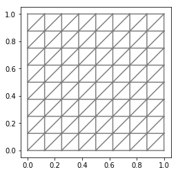
mesh = UnitSquareMesh(8, 8)
V = FunctionSpace(mesh, 'P', 1)
# Define boundary condition
u_D = Expression('1 + x[0]*x[0] + 2*x[1]*x[1]', degree = 2)
def boundary(x, on_boundary):
return on_boundary
bc = DirichletBC(V, u_D, boundary)
plot(mesh)
Define problem and compute solution
# Define variational problem
u = TrialFunction(V)
v = TestFunction(V)
f = Constant(-6.0)
a = dot(grad(u), grad(v))*dx
L = f*v*dx
# Compute solution
u = Function(V)
solve(a == L, u, bc)
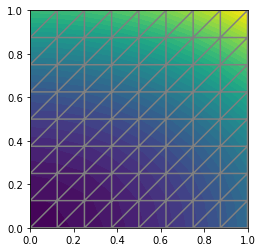
# Plot solution and mesh
plot(u)
plot(mesh)
errors
# Compute error in L2 norm
error_L2 = errornorm(u_D, u, 'L2')

# Compute maximum error at vertices
vertex_values_u_D = u_D.compute_vertex_values(mesh)
vertex_values_u = u.compute_vertex_values(mesh)
error_max = np.max(np.abs(vertex_values_u_D - vertex_values_u))

# Print errors
print('error_L2 = ', error_L2)
print('error_max = ', error_max)
error_L2 =  0.008235098073354827
error_max =  1.3322676295501878e-15