Compute the deflection $D(x,y)$ of a two-dimensional, circular membrane of radius $R$, subject to a load $p$ over the membrane.
Reference
PDE
\[-T\nabla^2 D=p \text{ in } \Omega = \{(x,y)|x^2 + y^2 \le R\}.\]Here $T$ is the tension in the membrane (constant), and $p$ is the external pressure load. The boundary of the membrane has no deflection (fixed), implying $D=0$ as a boundary condition. A localized load can be modeled as a Gaussian function:
\[p(x,y) = {A\over 2\pi\sigma} \exp\left(-{1\over 2}\left( {x-x_0\over \sigma}\right)^2 - {1\over 2}\left({y - y_0\over\sigma}^2\right)\right).\]$A$ is the ampitutde of the pressure, $(x_0, y_0)$ the localization of the maximum point of the load, and $\sigma$ the “width” of $p$. We will take the center $(x_0, y_0)$ of the pressure to be $(0, R_0)$ for some $0<R_0<R$.
Scaling the equation
\[-{\partial^2\omega\over\partial\bar{x}^2} - {\partial^2\omega\over\partial\bar{y}^2} = \alpha \exp\left(-\beta^2(\bar{x}^2 + (\bar{y} - \bar{R_0})^2)\right) \text{ for } \bar{x}^2 + \bar{y}^2 < 1,\]where
\[\alpha = {R^2 A\over 2\pi T D_c \sigma}, \beta = {R\over \sqrt{2} \sigma}.\]and $\bar{x} = x/R, \bar{y} = y/R, \omega = D/D_c, \bar{R_0} = R_0/R$, $D_c$ is a characteristic size of the deflection
In this case, $\alpha = 4, D_c = AR^2/(8\pi\sigma T)$ and droppint the bar we obtain the scaled problem
\[-\nabla^2\omega = 4\exp\left(-\beta^2 (x^2 + (y-R_0)^2)\right),\]with $\omega=0$ on the boundary, the dimensionless extent of the pressure $\beta\rightarrow 0$, the solution will approach the special case $\omega = 1-x^2-y^2$. The localization of the pressure peak, $R_0\in[0, 1].$
Given a computed scaled solution $\omega$, the physical delection ca be computed by
\[D = {AR^2\over 8\pi \sigma T} \omega.\]Variational formulation
PDE formulation
\[-\int_\Omega(\nabla^2 w) v\mathrm d x = \int_\Omega pv \mathrm d x.\]canonical notation
find $w\in V$ such that
\[a(w, v) = L(v) \quad \forall v\in\hat{V}.\]where
\[a(w, v) = \int_\Omega \nabla w\cdot \nabla v \mathrm d x, \\ L(v) = \int_\Omega pv \mathrm d x.\]Codes
settings
# enviroment setting

from fenics import *
from mshr import *
import numpy as np

import matplotlib.pyplot as plt
mesh
# define mesh
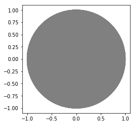
domain = Circle(Point(0, 0), 1)
mesh = generate_mesh(domain, 64)
V = FunctionSpace(mesh, 'P', 2)
plot(mesh)
boundary condition
# define boundary condition
w_D = Constant(0)

def boundary(x, on_boundary):
    return on_boundary

bc = DirichletBC(V, w_D, boundary)
load, variational problem and solution
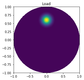
# define load

beta = 8
R0 = 0.6
p = Expression('4*exp(-pow(beta, 2)*(pow(x[0], 2) + pow(x[1] - R0, 2)))', degree = 1, beta=beta, R0=R0)

# define the variational problem

w = TrialFunction(V)
v = TestFunction(V)
a = dot(grad(w), grad(v))*dx
L = p*v*dx

# compute solution
w = Function(V)
solve(a == L, w, bc)
visualiztion
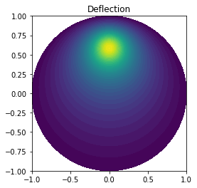
# plot deflection

plot(w, title='Deflection')
# plot load
plot(p, title='Load', mesh=mesh)
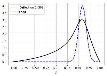
# curve plot along x = 0 comparing p and w

tol = 0.001
y = np.linspace(-1 + tol, 1 - tol, 101)
points = [(0, y_) for y_ in y]
w_line = np.array([w(point) for point in points])
p_line = np.array([p(point) for point in points])
plt.plot(y, 50*w_line, 'k', linewidth=2) # magnify w
plt.plot(y, p_line, 'b--', linewidth=2)
plt.grid(True)
plt.xlabel('$y$')
plt.legend(['Deflection ($\\times 50$)', 'Load'], loc='upper left')